PC Algorithm: Further examples

In the previous examples, we used a basic test data set to illustrate how to use the PC algorithm and how to visualise and interpret the results. The test data set was created using a simple linear model that followed the structure of the test DAG shown above. Depending on the field or discipline we are working in, we may encounter data sets whose components are not necessarily linearly related. It is hence worthwhile to analyse how the PC algorithm performs when working with more complex, nonlinear data sets:

using Distributions
using CausalInference
using TikzGraphs
# If you have problems with TikzGraphs.jl, 
# try alternatively plotting backend GraphRecipes.jl + Plots.jl
# and corresponding plotting function `plot_pc_graph_recipes`

N = 1000 # number of data points

x = rand(Uniform(0,2π), N)
v = sin.(x) + randn(N)*0.25
w = cos.(x) + randn(N)*0.25
z = 3 * v.^2 - w + randn(N)*0.25 
s = z.^2 + randn(N)*0.25

df = (x=x,v=v,w=w,z=z,s=s)

The data set created above exhibits the same causal structure, but now the individual variables are related to each other in a (deliberately) nonlinear fashion. As before, we can run the PC algorithm on this data set using the Gaussian conditional independence test:

plot_pc_graph_tikz(pcalg(df, 0.01, gausscitest), [String(k) for k in keys(df)])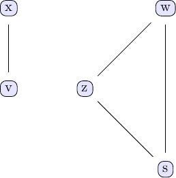

Interestingly enough, the resulting graph bears no resemblance to the true graph we would expect to see. To understand what's happening here, we need to remind ourselves that the PC algorithm uses conditional independence tests to determine the causal relationships between different parts of our data set. It seems as if the Gaussian conditional independence test we are using here can't quite handle the nonlinear relationships present in the data (note that increasing the number of data points won't change this!). To handle cases like this, we implemented additional conditional independence tests based on the concept of conditional mutual information (CMI). These tests have the benefit of being independent of the type of relationship between different parts of the analysed data. Using these tests instead of the Gaussian test we used previously is achieved by simply passing cmitest instead of gaussci as the conditional independence test to use to the PC algorithm:

plot_pc_graph_tikz(pcalg(df, 0.01, cmitest), [String(k) for k in keys(df)])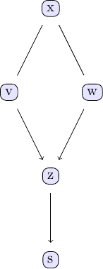

The result of the PC algorithm using the CMI test again look like what we'd expect to see. It should be pointed out here that using cmitest is significantly more computationally demanding and takes a lot longer than using gausscitest.