Reasoning about experiments

The following examples is discussed as Example 3.4 in Chapter 3-4 (http://bayes.cs.ucla.edu/BOOK-2K/ch3-3.pdf). See also http://causality.cs.ucla.edu/blog/index.php/category/back-door-criterion/.

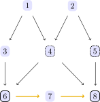
The causal model we are going to study can be represented using the following DAG concerning a set of variables [1,2,3,4,5,6,7,8]:

using CausalInference

dag = digraph([
    1 => 3
    3 => 6
    2 => 5
    5 => 8
    6 => 7
    7 => 8
    1 => 4
    2 => 4
    4 => 6
    4 => 8])
t = plot_pc_graph(dag)

We are interested in the average causal effect (ACE) of a treatment X=[6] on an outcome Y=[8], which stands for the expected increase of Y per unit of a controlled increase in X.

Regressing Y=[8] on X=[6] will fail to measure the effect because of the presence of a confounder C[4], which opens a backdoor path, a connection between X and Y via 6 ← 4 → 8 which is not causal.

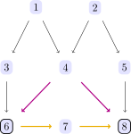
We can avert such problems by checking the backdoor criterion. Indeed

backdoor_criterion(dag, 6, 8) # false

reports a problem.

One might want to condition on the confounder C = [4] to obtain the causal effect, but then

backdoor_criterion(dag, 6, 8, [4]) # still false

there is still a problem ( because that conditioning opens up a non-causal path via 6 ← 3 ← 1 → 4 ← 2 → 5 → 8.)

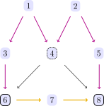
But conditioning on both Z = [3, 4] solves the problem, as verified by the backdoor criterion.

backdoor_criterion(dag, 6, 8, [3,4]) # true
backdoor_criterion(dag, 6, 8, [4,5]) # true

(also conditioning on Z = [4, 5] would be possible.)

Thus, regressing Y=[8] on X=[6] and controlling for Z=[3, 4] we measure the average causal effect.